Quick Start Guide
Prerequisites
there are none, but its good to know std/pine syntax (gonna implement c style syntax soon enough fs cus thats just better)
Step 1
step 1: initialize the indicator by giving it a name and specifying the overlay status (if it should be in its own pane or not)
//    Description,  display name, overlay
indicator("Indicator", "dih", false)
Step 2
step 2: this is where you kinda go your own way, but if you dont know what to do this tutorial will go over how to use some ifs and technical analysis statements to plot something, idk what rn we'll se what ends up happening
anyways, let's add a simple rsi line:
let rsi = ta.rsi(close, 14)
if you're a noob then lemme explain what each part of that does:
let rsi - this initializes a new variable with name "rsi", obviously.
= ta.rsi(close, 14) - give the variable a value, in this case, we call ta.rsi() with some inputs: close and 14 - the former meaning the source (open/high/low/close/volume/etc) and the latter the "length" (how many bars back ta.rsi() uses to calculate the rsi)
Step 3
now that we've initialized a new indicator, and gotten a value to plot, lets plot it!
plot(rsi)
and thats about it. full code:
indicator("Indicator", "dih", false)

let rsi = ta.rsi(close, 14)

plot(rsi)
simple, right? You should now see something like this:
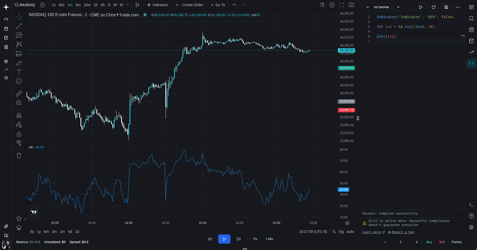
if you do, then you did everything right! if not, you failed a very simple task and should consider not continuing this tutorial
anyways, let's add some more stuff!
Step 4
let's add some bounds
//hline creates a horizontal line on the chart (obviously)
//also, let's save the return value from hline to variables (hline1, hline2)
let hline1 = hline(70) //hline takes in a price as the first argument
let hline2 = hline(30) //^
and a fill between them:
//fill fills an area (only between hline-hline / plot-plot)
fill(hline1, hline2, color.purple) //takes in two plots or -
//two hlines as first two arguments, then a color
looks better now, but still ahh. so, let's add an overbought and oversold gradient!
//for this, we'll need to use a fill()

//define levels for the fill
let hline100 = hline(100)
let hline70 = hline(70)

fill(hline100, hline70, 100, 70,
top_color=color.new(color.green, 0), bottom_color=color.new(color.green, 100))

//color.new(color.green, 0) is creating a new green color,
// with transparency 0 (opaque)
//color.new(color.green, 100) is creating a new green color,
// with transparency 100 (fully transparent)
wait! this looks new - what is "100, 70" and the rest!? look closely - we dont use "color=xx" but "top_color=xx" and "bottom_color=xx". So what "100, 70" does is that it's defining levels for the gradient - top level (in this case 100) and bottom level (in this case 70).
why? why not just use the value of the plots/hlines as top/bottom level? that would work fine for hlines, but lets say a plot's price is increasing in value constantly (y=x) against a static horizontal plot, the gradient would be tilted 45 degrees! (this will become even more apparent later on)
so now, this produces this:
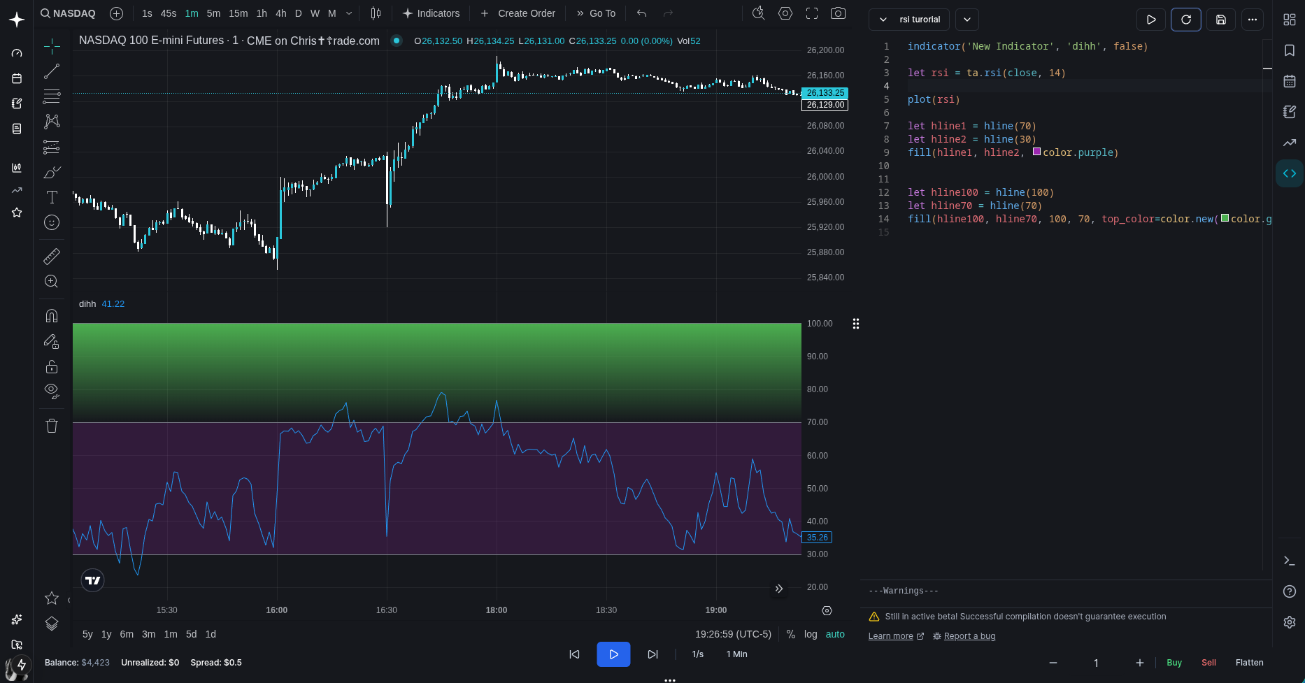
hold on. this is not right at all!
What is this!!! 😡😡
let's look at the code again:
let hline100 = hline(100)
let hline70 = hline(70)
fill(hline100, hline70, 100, 70,
top_color=color.new(color.green, 0), bottom_color=color.new(color.green, 100))
ah, right. think i found it - we're creating a gradient between prices 100 and 70 - but what we actually want is between the actual rsi and ... the upper bound (price 70)?
let's try doing that to see if it fixes the issue:
//first, we need to make this line:
plot(rsi)

//into this:
let rsiPlot = plot(rsi)
//because we need a reference to the plot to use in the fill function
and now, let's update the rest:
//first, remove these two:
let hline100 = hline(100)
let hline70 = hline(70)

//secondly - add this:
let midlinePlot = plot(50, editable=false, display=display.none)
//why? because we need two plots in the fill() function!
//we could make it plot(70), but you'll see why we made it 50 soon
//we also add "editable=false" to hide it in the indicator settings
//and also display=display.none so that its not visible

//lastly, update this fill() call:
fill(hline100, hline70, 100, 70,
top_color=color.new(color.green, 0), bottom_color=color.new(color.green, 100))

//so that it becomes this:
fill(rsiPlot, midlinePlot, 100, 70,
top_color=color.new(color.green, 0), bottom_color=color.new(color.green, 100))

//remember when i was talking about the 45 degrees stuff?
//here's where you learn why we put top and bottom values -
//right now the gradient would go down from the rsi value down to the midline value
//(50) but we want it to end at 70, so we put the bottom value as 70
// so that it's bottom level becomes 70 (you can tweak this if you want :)
so let's try it out now..
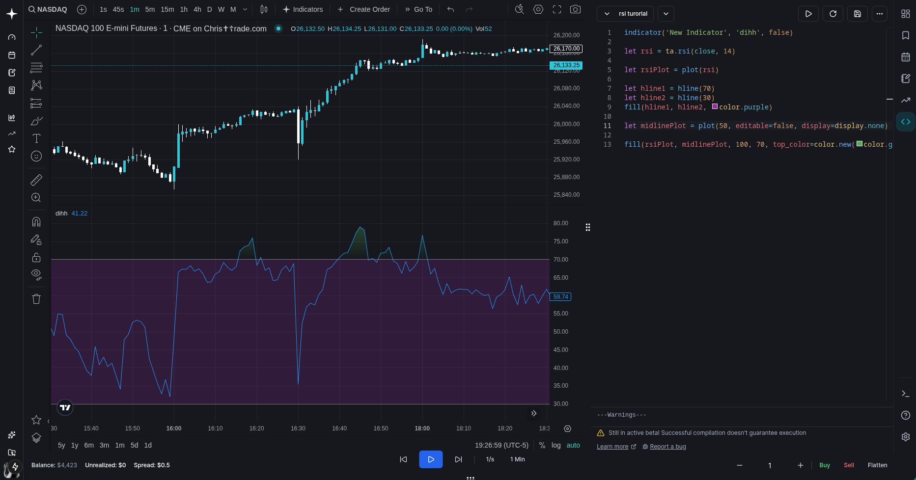
yeah! that's more like it!!
let's make it look a bit nicer, and also, if you're lost, let me provide you with the full code:
indicator('New Indicator', 'dihh', false)

let rsi = ta.rsi(close, 14)

let rsiPlot = plot(rsi, color=color.purple, linewidth=1)

//added linestyle=hline.style_dashed to the bounds hlines
let hline1 = hline(70, linestyle=hline.style_dashed)
let hline2 = hline(30, linestyle=hline.style_dashed)
fill(hline1, hline2, color.new(color.purple, 90))

let midlinePlot = plot(50, editable=false, display=display.none)

fill(rsiPlot, midlinePlot, 100, 70,
top_color=color.new(color.green, 0), bottom_color=color.new(color.green, 100))
oh yeah, and let's also add an oversold gradient, you should be able to understand all the parts here by now (i hope)
fill(rsiPlot, midlinePlot, 30, 0,
top_color=color.new(color.red, 100), bottom_color=color.new(color.red, 0))
what now...? let's add a moving average:
//add this under let rsiPlot = plot(rsi, color=color.purple, linewidth=1)

//ta is short for technical analysis, it has a lot of built in calculations like
// ema, sma, rsi, macd, percentile linear interpolation (whatever the hell that is)
//  etc etc etc (a lot of stuff basically)

//ta.sma() takes two arguments: source & length - for this example,
// it calculates the average of the past 14 rsi values pretty much
let rsiMa = ta.sma(rsi, 14)
//and then plot it of course and give it a nice color
plot(rsiMa, color=color.yellow)
yeah yeah more comments than code i know but im trying here alright
anyways, now it looks pretty nice!
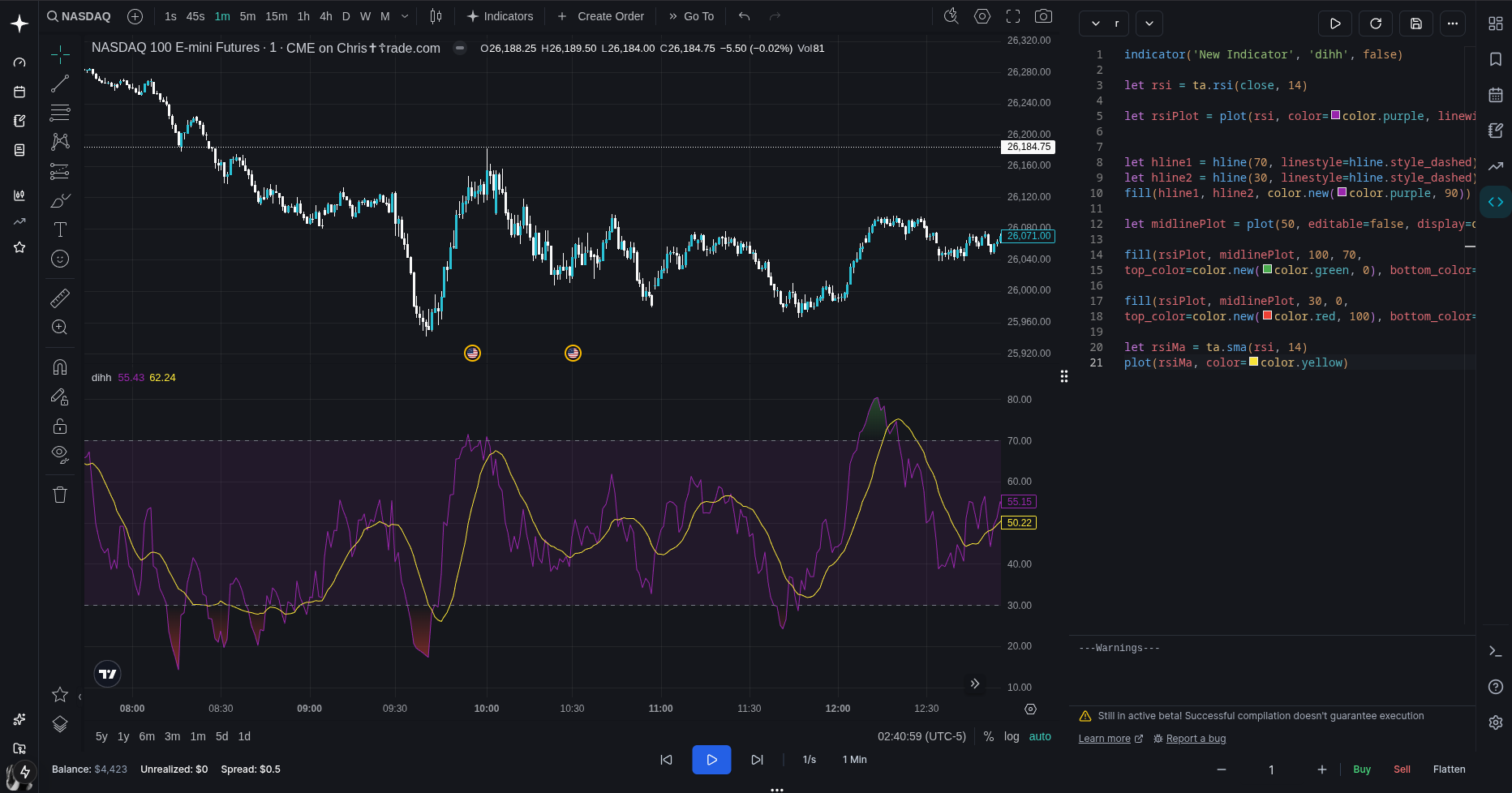
but i feel there is one thing missing... divergences!
Step 5
thus far the code has been super simple. here's where it gets more complex, so strap in, but first - what even is a divergence? its basically when two things diverge. Let's say price is in a downtrend and keeps making lower lows and lower highs, but the rsi is in an uptrend - making higher lows and higher highs. take a guess what we got there (hint: it starts with "divergence"). Remember, divergences exist across everything so dont limit it to price vs rsi - it could be price vs volume, open vs close etc etc (but not every combo is equally meaningful)
But why is that useful? Well let's ask this: what happens before a reversal? often when price diverges from something - it could be volume, volatility, momentum, etc (and since rsi is calculated based on price movement, it could indicate price reversing). Not with 100% accuracy of course, but it could be a confluence
Anyways, enough talking and lets go back to the code.
so where do we even start? check if price is trending and then if the rsi is not/not in the same direction? Yes
Let's start of by checking for bullish divergences (price trending down and rsi not trending down)
// how far to look to the right of a pivot.
// right = future bars, so this basically delays confirmation
lookbackRight = 5

// how far to look to the left of a pivot.
// left = past bars, so this controls how "clean" the swing needs to be
lookbackLeft = 5

// max bars between two pivots to still call it a divergence
rangeUpper = 60

// min bars between two pivots (ignore tiny noise pivots 1-5 bars apart etc)
rangeLower = 5

// did we just find an rsi pivot low on this bar
plFound = false

// final "yes/no" flag for bullish divergence
bullCondition = false
okay that was simple. now the hard stuff comes. you'll now learn how to look back in time and create functions! yay!
// rsi value at the potential pivot bar (lookbackRight bars back from now)
// pivot is always confirmed after lookbackRight bars, so we grab that bar's rsi
rsiLBR = rsi[lookbackRight]

//hold on! what is [lookbackRight]? what does [] do?
//well it looks back in time of course! right now lookbackRight = 5,
//so we're checking rsi's value 5 bars back - easy right!

// helper function (whoa now we learn how to create a function!)
// to make sure the distance between pivots is within our range
// that was true on pivot bars (in our case plFound[1])
// condition = some bool (boolean means true or false)
isInRange(bool condition) =>
    // how many bars since the last time 'condition' was true
    bars = ta.barssince(condition)
    // only allow divergences where the pivots are not too close or too far apart
    // then return true if it is, or false if not
    rangeLower <= bars and bars <= rangeUpper

// detect an rsi pivot low:
// ta.pivotlow(series, left, right) returns a value ONLY on the pivot bar, else na
// (na means not applicable/available - basically undefined/NaN)
// so if it's not na, we just confirmed a pivot low on rsi
plFound := not na(ta.pivotlow(rsi, lookbackLeft, lookbackRight))

//wait what is :=?
//it reassigns a variable! so whenever you need to change an existing variable's
//value, use :=

// check if rsi made a higher low
// rsiLBR = current pivot's rsi (the one we just found)
// ta.valuewhen(plFound, rsiLBR, 1) = rsiLBR value at the previous pivot low
// isInRange(plFound[1]) makes sure the current and previous pivots are within range
rsiHL = rsiLBR > ta.valuewhen(plFound, rsiLBR, 1) and isInRange(plFound[1])

// grab the price low at the same pivot bar (lookbackRight bars ago)
lowLBR = low[lookbackRight]

// check if price made a lower low compared to the previous pivot low
// ta.valuewhen(plFound, lowLBR, 1) = previous pivot's low price
priceLL = lowLBR < ta.valuewhen(plFound, lowLBR, 1)

// now we finally say bullish divergence exists if:
// 1) we have a pivot low now (plFound)
// 2) price made a lower low (priceLL)
// 3) rsi made a higher low (rsiHL)
// classic regular bullish divergence: price ↓, rsi ↑
//and then set bullCondition to that!
bullCondition := priceLL and rsiHL and plFound

//now we've determined if we got a bullish divergence, time to plot it!
plot(
     // only plot something when we actually have a pivot
     // if you dont know what "? :" means - it's called turnary
     // if plFound is true, we plot rsiLBR; if plFound is false, we plot na
     plFound ? rsiLBR : na,
     // shift the plot back so it lines up with the actual pivot bar,
     // not the bar where it finally got confirmed
     offset = -lookbackRight,
     title = "Bullish Divergence",
     linewidth = 2,
     // if we have an actual bullish divergence, paint it green
     // otherwise make it invisible (fully transparent white)
     color = (bullCondition ? color.green : color.new(color.white, 100)),
     // put this in the RSI pane, not on price
     display = display.pane)
Alright! That wasnt so hard was it? I do recommend reading it over a couple times to get it, but the principle itself is pretty simple.
so now we should have something like this:
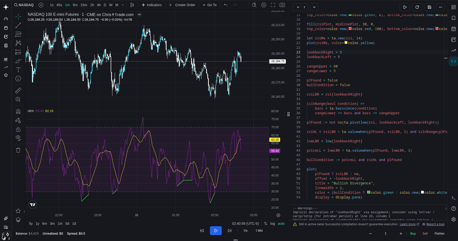
see the green lines? That means it's working! If you dont have them you probably did something wrong :( (idk how you would even manage to do that this is literally a step by step tutorial lol)
Now let's implement bearish divergences - but first, try to do this yourself as you'll learn a lot, i promise. If you tried and couldnt get it working, let me help you out
//implementing bearish divergences is pretty much the same process but reversed
//so i'll go easier on the comments this time - you'll understand by now im sure

//first add these among the others:
phFound = false
bearCondition = false

//then, under this line: bullCondition := priceLL and rsiHL and plFound
//add this:
phFound := not na(ta.pivothigh(rsi, lookbackLeft, lookbackRight))
rsiLH = rsiLBR < ta.valuewhen(phFound, rsiLBR, 1) and isInRange(phFound[1])
highLBR = high[lookbackRight]
priceHH = highLBR > ta.valuewhen(phFound, highLBR, 1)
bearCondition := priceHH and rsiLH and phFound

//this is doing pretty much the same calculations as before,
//just inversed (pivothigh instead of pivotlow,
//high[lookbackRight] insted of low[lookbackRight],
// < becomes >, > becomes < and lowLBR becomes highLBR)

//lastly, add this to plot the bearish divergences:
plot(
    phFound ? rsiLBR : na,
    offset = -lookbackRight,
    title = "Bearish Divergence",
    linewidth = 2,
    color = (bearCondition ? color.red : color.new(color.white, 100)),
    display = display.pane)
If you did everything right, you should now see this:
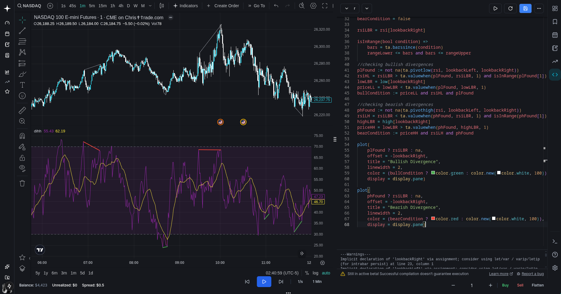
And as you can see, it's working super well! Sadly this tutorial is coming to an end, but first i just want to add one more thing:
//add these two at the end of the code
//they add nice labels next to the rsi lines
//the code should be pretty self-explaining by now
plotshape(
     bullCondition ? rsiLBR : na,
     offset = -lookbackRight,
     title = "Bullish Label",
     text = "Bull",
     style = shape.labelup,
     location = location.absolute,
     color = color.green,
     textcolor = color.white,
     display = display.pane)

plotshape(
     bearCondition ? rsiLBR : na,
     offset = -lookbackRight,
     title = "Bearish Label",
     text = "Bear",
     style = shape.labeldown,
     location = location.absolute,
     color = color.red,
     textcolor = color.white,
     display = display.pane)
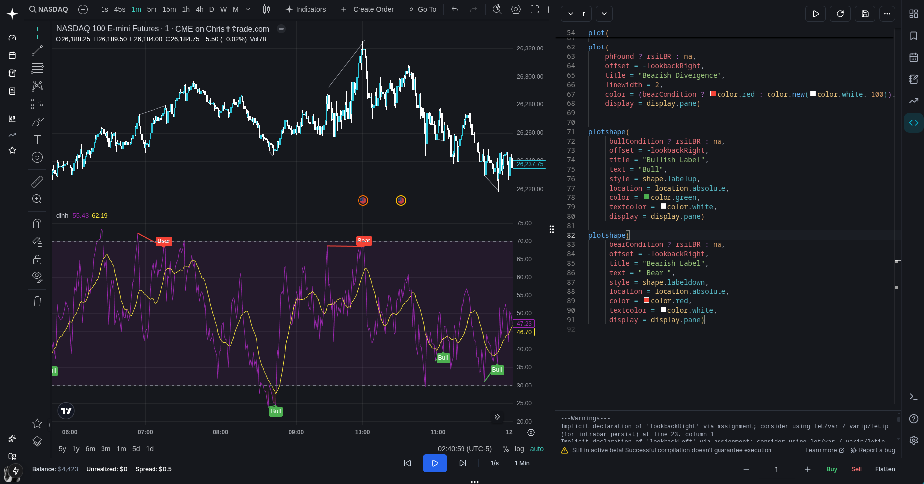
much better!
oh yeah! full code:
indicator('New Indicator', 'dihh', false)

let rsi = ta.rsi(close, 14)

let rsiPlot = plot(rsi, color=color.purple, linewidth=1)


let hline1 = hline(70, linestyle=hline.style_dashed)
let hline2 = hline(30, linestyle=hline.style_dashed)
fill(hline1, hline2, color.new(color.purple, 90))

let midlinePlot = plot(50, editable=false, display=display.none)

fill(rsiPlot, midlinePlot, 100, 70,
top_color=color.new(color.green, 0), bottom_color=color.new(color.green, 100))

fill(rsiPlot, midlinePlot, 30, 0,
top_color=color.new(color.red, 100), bottom_color=color.new(color.red, 0))

let rsiMa = ta.sma(rsi, 14)
plot(rsiMa, color=color.yellow)

lookbackRight = 5
lookbackLeft = 5

rangeUpper = 60
rangeLower = 5

plFound = false
phFound = false
bullCondition = false
bearCondition = false

rsiLBR = rsi[lookbackRight]

isInRange(bool condition) =>
    bars = ta.barssince(condition)
    rangeLower <= bars and bars <= rangeUpper

//checking bullish divergences
plFound := not na(ta.pivotlow(rsi, lookbackLeft, lookbackRight))
rsiHL = rsiLBR > ta.valuewhen(plFound, rsiLBR, 1) and isInRange(plFound[1])
lowLBR = low[lookbackRight]
priceLL = lowLBR < ta.valuewhen(plFound, lowLBR, 1)
bullCondition := priceLL and rsiHL and plFound

//checking bearish divergences
phFound := not na(ta.pivothigh(rsi, lookbackLeft, lookbackRight))
rsiLH = rsiLBR < ta.valuewhen(phFound, rsiLBR, 1) and isInRange(phFound[1])
highLBR = high[lookbackRight]
priceHH = highLBR > ta.valuewhen(phFound, highLBR, 1)
bearCondition := priceHH and rsiLH and phFound

plot(
    plFound ? rsiLBR : na,
    offset = -lookbackRight,
    title = "Bullish Divergence",
    linewidth = 2,
    color = (bullCondition ? color.green : color.new(color.white, 100)),
    display = display.pane)

plot(
    phFound ? rsiLBR : na,
    offset = -lookbackRight,
    title = "Bearish Divergence",
    linewidth = 2,
    color = (bearCondition ? color.red : color.new(color.white, 100)),
    display = display.pane)


plotshape(
     bullCondition ? rsiLBR : na,
     offset = -lookbackRight,
     title = "Bullish Label",
     text = "Bull",
     style = shape.labelup,
     location = location.absolute,
     color = color.green,
     textcolor = color.white,
     display = display.pane)

plotshape(
     bearCondition ? rsiLBR : na,
     offset = -lookbackRight,
     title = "Bearish Label",
     text = "Bear",
     style = shape.labeldown,
     location = location.absolute,
     color = color.red,
     textcolor = color.white,
     display = display.pane)
I really hope you learnt something, this code is not that complicated(only 90 lines, you should see the amount of code needed to compile this hahah) so yeah i might do another tutorial in the future if someone wants it
man kinda sad its over now :( but i do hope you learnt something - you should definitely try changing stuff to really learn how it works
also, this tutorial didnt cover how to add inputs in the indicator settings like when you double click it, that's something for you to do :)
But yeah that's about it, thank you so much for reading! and bye!!